Coursera Machine Learning Week 10-11

Contents: More types of gradient descent, online learning, pipeline and more

Gradient descent

Batch Gradient descent: using the whole dataset in every iteration

Stochastic gradient descent

Unlike Batch Gradient descent, this approach uses only one example in one iteration. Here is how it works:

1. Randomly shuffle (reorder) training examples
2. Repeat one or several times {
   for i = 1,…,m
         $\theta_j := \theta_j - \alpha (h_\theta(x^{(i)}) - y^{(i)}) x^{(i)}_j$ for j = 1,…,n
   }
3. Everything else is the same as in Batch gradient descent

Stochastic gradient descent is often not going to reach global minimum, but instead ends up wandering around it’s neighboring area. This is not a big problem in practice as long as it is close enough.

Mini-batch gradient descent

So far we have seen two types of gradient descent, here we introduce the final one by comparing them:

• Batch gradient descent: Use all m examples in each iteration
• Stochastic gradient descent: Use 1 example in each iteration
• Mini-batch gradient descent: Use b examples in each iteration

This approach works as following:

1. Let b = 10, say.
2. Randomly shuffle (reorder) training examples
3. Repeat one or several times {
   for i = 1,11,21,…,m-9
         $\theta_j := \theta_j - \frac{\alpha}{10} \sum^{10}_{k=1} (h_\theta(x^{(k)}) - y^{(k)}) x^{(k)}_j$ for j = 1,…,n
   }
4. Everything else is the same as in Batch gradient descent

Mini-batch gradient descent allows us to perform vertorization, which leads to higher efficiency such that it may work even faster than the Stochastic one.

Gradient descent convergence

With batch gradient descent, we plot cost at each iteration against no. iterations to check convergence. For the other two types of gradient descent, similar idea is applied.

We take stochastic gradient descent as example. Here is the cost function for it:

$$cost (\theta, (x^{(i)}, y^{(i)})) = \frac{1}{2} (h_\theta(x^{(i)}) - y^{(i)})^2$$

It’s certainly not a good idea to plot it against no. iteration straight away. So instead, we use the cost averaged over the last i examples:

$$\frac{1}{i} \sum_{k=1}^icost (\theta, (x^{(k)}, y^{(k)}))$$

This gives a better view of how the algorithm has performed on last i examples, so we should be able to check convergence.

Learning rate

Normally, like cost of batch gradient descent, the averaged cost going downwards gently as no. iteration increases, but learning rate can have effects on it:

We see that with smaller learning rate, the algorithm can end up with slightly better result, but note that smaller learning rate would slow the speed of convergence. Moreover, in the case that the averaged cost is going upwards (indicates divergence), making learning rate smaller would also help.

On the other hand, if we want θ to converge, then rathen than holding learning rate constant, we can slowly decrease α over time to do so:

$$\alpha = \frac{c_1}{c_2 + \text{no. interation}}$$

where $c_1, c_2$ is the additional parameters we need to mannually manipulate with.

Online learning

Online learning algorithms has a property that each example is processed only once, such that it usually best suited to problems were we have a continuous/non-stop stream of data that we want to learn from.

The approach works like this:

Repeat forever {
get information from new user (x, y)
Update θ using (x, y):
      $\theta_j := \theta_j - \alpha (h_\theta(x) - y) x_j$ for j = 1,…,n
}

So the algorithm keep updating θ whenever new x comes in. It’s easy to imagine the possible application scenarios: Choosing special offers to show user; customized selection of news articles; product recommendation. The course gives a detailed example to show how it can be applied:

Product search (learning to search)

• User searches for “Android phone 1080p camera”
• Have 100 phones in store. Will return 10 results.
• x = features of phone, how many words in user query match name of phone, how many words in query match description of phone, etc.
• y = 1 if user clicks on link. y = 0 otherwise.
• Learn $p(y = 1\vert x;\theta)$ (also called the predicted click through rate (CTR))
• Use to show user the 10 phones they’re most likely to click on.

One advantage of online learning if the function we’re modeling changes over time (such as if we are modeling the probability ($p(y\vert x;\theta)$) of users clicking on different URLs, and user tastes/preferences/ are changing over time), the online learning algorithm will automatically adapt to these changes.

Map-reduce and data parallelism

No fancy things in this topic, so I will only write a short introdction:

Map-reduce basically means use more than one computer to calculate the summation part, so for example if we sum over 400 examples, just let 4 computers to do 100 of them respectively. Similarly, data parallelism just means apply multithreading stuff to the calculation.

I know you are thinking what a lazy guy I am, so here is a detailed version with Q&A related to big data that I strongly recommended.

Week 11

Pipeline

Having a complex machine learning problem is common in the real world, where there is not a easy way to solve it. So it is usually helpful to divide the problem into several components such that we can then work on them part by part. Such technique of building a system with many stages / components, several of which may use machine learning is called a pipeline.

The course gives an example of Photo OCR(photo optical character recognition), where it was divided into four components:

• Image
• Text detection
• Character segmentation
• Character Recognition

Text detection is the part where the course spent most of time with, the ideas of sliding windows and expansion algorithm were introduced.

Artificial data synthesis

This technique is one way of getting a large amount of training examples, where we are trying to make new examples artificially by simulating / modifying the original ones. E.g. Character Recognition:

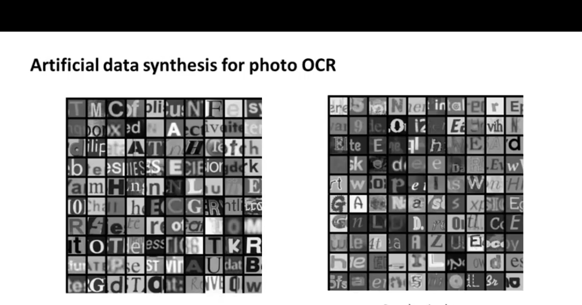
Based on the graph on the left, we can manually create new examples by using different fonts, paste these characters in random backgrounds and apply blurring/distortion filters, which shows on the right.

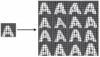
Another way is to modify the original example by, for example, warping it:

Ceiling analysis

Ceiling analysis is a way to guide you which part of the pipeline to work on next. It can help indicate that certain components of a system might not be worth a significant amount of work improving, because even if it had perfect performance its impact on the overall system may be small. Therefore it helps us decide on allocation of resources in terms of which component in a machine learning pipeline to spend more effort on.
We take Photo OCR as example again:

Component	Accuracy
Overall performance	70%
Text detection	85%
Character segmentation	89%
Character Recognition	100%

It might be unclear what is going on in the above, so I take the text detection part to explain: after using correct answer straight away instead of machine learning algorithm, the accuracy increases from 70% to 85%.

So there is a large gain in performance possible in improving the text detection and character recognition part, and we should not spend too much time on improving character segmentation.

Note that performing the ceiling analysis shown here requires that we have ground-truth labels for the text detection, character segmentation and the character recognition systems.