Coursera Machine Learning Week 8

Contents: Unsupervised learning algorithm —- K-means and Principal Component Analysis

Unsupervised learning allows us to approach problems with little or no idea what our results should look like. We can derive structure from data where we don’t necessarily know the effect of the variables.

K-means algorithm

K-means clustering is the fisrt unsupervised algorithm that we are going to learn, it aims to partition n observations into k clusters in which each observation belongs to the cluster with the nearest mean, serving as a prototype of the cluster.

Input:

• K — Number of clusters
• Training Set {$x^{(1)}, x^{(2)}, ..., x^{(m)},$}, where $x^{(i)} \in \mathbb{R}^n$. Note that we don’t need the bias term $x_0=1$ here.

Cost function

Firstly let:

• $c^{(i)}$ = index of cluster (1, 2, .., K) to which example $x^{(i)}$ is currently assigned
• $\mu_k$ = cluster centroid k ( $\mu_k \in \mathbb{R}^n$)
• $\mu_{c^{(i)}}$ = cluster centroid of cluster to which example $x^{(i)}$ has been assigned

Then the cost can be written as:

$$J(c^{(1)},...,c^{(m)}, \mu_1, ..., \mu_K) = \frac{1}{m} \sum^m_{i=1} \|x^{(i)}-\mu_{c^{(i)}}\|^2$$

Random initialization

We initialize clusters by randomly pick K traning examples, then set $\mu_1, \mu_2, ..., \mu_K$ equal to these examples. Formally:
Pick k distinct random integers $i_1, ..., i_k$ from {1, .., m}, then set $\mu_1 = x^{(i_1)}, \mu_2 = x^{(i_2)}, ..., \mu_k = x^{(i_k)}$.

Optimizating objective

Next, in order to minimise the cost function, we find the appropriate values of $c^{(1)},...,c^{(m)}, \mu_1, ..., \mu_K$ through the following iteration:

---

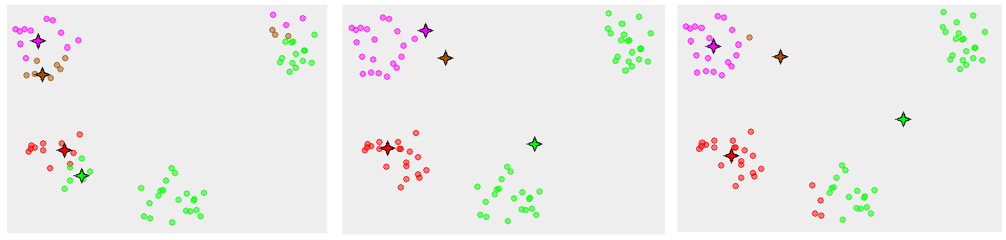
Randomly initialize K cluster centroids $\mu_1, \mu_2, ..., \mu_K \in \mathbb{R}^n$

Repeat {

• for i = 1 to m
  $\ \ \ \ \ \ c^{(i)}$ := index of cluster centroid closest to $x^{(i)}$, where $c^{(i)} \in \mathbb{N}^K$.

• for k = 1 to K
  $\ \ \ \ \ \ \mu_k$ := average of points assigned to cluster k, namely:$\mu_k := \frac{1}{\text{number of }j} \sum_{j: c^{(j)} = k} x^{(j)}$.

  }

---

The first for loop is the clusters assignment step, where it’s minimising J by reassigning $c^{(i)}$ ‘s to closest clusters, holding $\mu_k$ ‘s fixed, while the second for loop is minimising J by moving centroids, leaving $c^{(i)}$ unchanged. So the cycle continues until the algorithm converges to the global minimum, and… what if it’s a local minimum?

For above we see there are many case where the K-means gives unexpected results, one way to solve this is to rerun the algorithm many times with different initializations, a pseudo code looks like:

for i = 1 to 100 {
    Randomly initialize K
    Run K-means to get c_1, ..., c_m, μ_1, ..., μ_K.
    Compute cost function J
}
Pick clustering that gave lowest J

Remeber that when testing the cross validation set, make sure use PCA first, then
apply the algorithm.

Choosing the value of K

How many clusters? A hard question. It’s the most common case that people choose it manually, but here is a little trick that you might consider to use — the Elbow method

Consider the image above as a part of human body: the highest point is the shoulder, the lowest is the hand, and the point surrounded by red circle is the elbow. It’s suggested that we shall choose the elbow point to decide how many clusters to use, as all the marginal costs after this point become insignificant and so are unnecessary.

On the other hands, you sometimes may run K-means to get clusters to use for some later/downstream purpose (e.g. sizes of T-shirt — S,M,L or XS, S, M, L, SL?), and evaluate K-means based on a metric for how well it performs for that later purpose.

Principal Component Analysis

PCA is a powerful unsupervised algorithm that can reduce data from n dimensions(features) to k dimensions, I will introduce it directly by showing how it works:

• Apply mean normalization and/or feature scaling to the dataset (important)

• Compute the n × n “covariance matrix”:

$$\begin{align*} \Sigma =& \ \frac{1}{m} \sum_{i=1}^{m} (x^{(i)})(x^{(i)})^T, \text{where}\ x^{(i)} \in \mathbb{R}^{n×1}, \text{or} \newline =& \ \frac{1}{m} X^T X, \text{where} \ X \in \mathbb{R}^{m×n} \end{align*}$$

• Computer the eigenvector U of the matric Σ:

$$U = \begin{bmatrix}\vert & \vert & & \vert \\ u^{(1)} & u^{(2)} & \dots & u^{(n)}\\ \vert & \vert & & \vert \end{bmatrix} \in \mathbb{R}^{n×n}$$

• From the matrix U, select first k columns as $U_{reduced} \in \mathbb{R}^{n×k}$, then get our $i_{th}$ example with new dimensions:

$$z^{(i)} = \begin{bmatrix}\vert & \vert & & \vert \\ u^{(1)} & u^{(2)} & \dots & u^{(k)}\\ \vert & \vert & & \vert \end{bmatrix}^T x^{(i)}= U_{reduced}^T x^{(i)} \in \mathbb{R}^{k×1}$$

• Or if we want specific $j_{th}$ feature, just use $z_j = (u^{(j)})^T x$

In matlab, we can get the eigenvectors and new example z as following:

[U,S,V] = svd(Sigma);
Ureduce = U(:,1:k);
z = Ureduce'*x;

PCA VS. Linear Regression

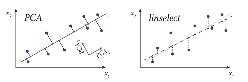
These two algorithms looks somehow similar but actually different. PCA is trying to minimising the following:

$$\frac{1}{m}\sum_{i=1}^m\|x^{(i)}-x^{(i)}_\text{approx}\|^2$$

While Linear Regression has a goal of minimising:

$$\frac{1}{m} \sum_{i=1}^m (h(x^{(i)}) - y^{(i)})^2$$

We can also see the difference from the graph below:

Choosing k (number of principal components)

When discussing PCA, rather than ask “what’s your value for k” , people would say “how many % of variance have you retained”. That means a strategy of choosing k by the following:

• Try PCA with k = 1
• Check if $\frac{\frac{1}{m}\sum_{i=1}^m\|x^{(i)}-x^{(i)}_\text{approx}\|^2}{\frac{1}{m}\sum_{i=1}^m\|x^{(i)}\|^2} \leq 0.01$
• if the above holds, then exits with current value of k. Otherwise, continue the loop with k += 1

So we end up with the smallest possible value of k that retained 99% of variance， it’s totally fine to choose other number like 95% instead of 99%. Note that the formula above is the same as $1 - R^2$ (1 - Coefficient of determination).

Moreover, we can obtain this value by using the matrix S provided by the function svd() used above:

[U,S,V] = svd(Sigma);

The S matrix will be a n by n matrix, and we have the procedure with exactly the same result:

Pick smallest value of k which makes 99% of variance retained:

$$\frac{\sum_{i=1}^k S^{ii}}{\sum_{i=1}^n S^{ii}} \geq 0.99$$

Application

There are two main use of PCA:

• Compression —- For the purpose of reducing memory/disk needed to store data, or in order to speed up learning algorithm.

• Visualization —- Reduce from a large nummber to 2 or 3 dimensions helps to extract the information and is able to visualize to show potential relationship.

However, it’s not a good use of PCA to try to prevent overfitting. It is true that fewer features makes overfit less likely to happen, but the loss of information may worse the performance. Instead, it is more reasonable to use regularization to do so.