Coursera Machine Learning Week 7

Contents: Support Vector Machine

BAD NEWS: Sadly, Couresara is no longer providing reading notes from this chapter and onwards for some reason (e.g. laze). That means I have to make the ENTIRE note by myself.

Week 7

Support Vector Machine

Cost function

The cost function for SVM is somehow similar to the one for logistic regression, such that we can get it by only editing a few things on the later one:

• replace $-\log h_\theta(x^{(i)})$ and $-\log (1 - h_\theta(x^{(i)})$ by $cost_1(\theta^T x^{(i)})$ and $cost_0(\theta^T x^{(i)} )$ respectively:

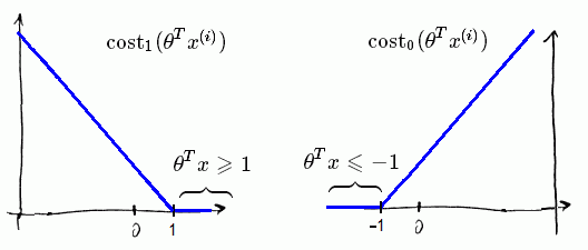
• multiply the whole function by m
• instead of multiply λ on the regularized term, we multiply a constant C on the data set terms (so that if C = $\frac{1}{\lambda}$, this edition has little effect)

So here is the brand new cost function:

$$\min_\theta C \ \sum_{i=1}^m [y^{(i)} cost_1(\theta^T x^{(i)}) + (1-y^{(i)}) \ cost_0(\theta^T x^{(i)})] + \frac{1}{2} \sum_{j=1}^{n}\theta_j^2$$

And in order to minimise the cost function, we want $\begin{align*} & \theta^T x^{(i)} \geq 1\quad \mbox{if}\ y^{(i)} = 1\\ & \theta^T x^{(i)} \leq -1\quad \mbox{if}\ y^{(i)} = 0 \end{align*}$.

SVM is a Large margin classifier, by this I mean the algorithm is trying to seek a decision boundary such that the distances between different groups of observations and the oundary are maximised. The following explain this mathematically:

Firstly, it can be shown that $\theta^T x^{(i)} = \|\theta\|\cdot p^{(i)}$, where $p^{(i)}$ is the projection of $x^{(i)}$ onto $\theta$, the graph below shows two examples of $p^{(i)}$:

Remeber that we are trying to minimise the cost function. Using the substitution above our goal is make $\begin{align*} & \|\theta\|\cdot p^{(i)} \geq 1\quad \mbox{if}\ y^{(i)} = 1\\ & \|\theta\|\cdot p^{(i)} \leq -1\quad \mbox{if}\ y^{(i)} = 0 \end{align*}$, that is to maximise $p^{(i)}$ by manipulating θ. The graph below shows a much better choice than the last one:

On the other hand, making $p^{(i)}$ large allows us to make θ small, as there is also another term in the cost function: $\frac{1}{2} \sum_{i=1}^n \theta_i^2$, or equvalently, $\frac{1}{2} \|\theta\|$.

Therefore it is clear that when C is getting large, the cost function becomes sensitive to the dataset, and thus sensitive to the outliers:

I understand there is a lack of details in the above description, and I do strongly recommend you to go to have a look at a detailed version that I found online.

Kernel

SVM is powerful to find non-linear boundaries, the secret behind it is called Kernel, all that about is the similarity function:

Previously, our hypothesis was written as

$$h_\theta(X) = \theta_0 + \theta_1 x_1 + \theta_2 x_1x_2 + \theta_3 x_2^2 + ...$$

It’s then generalized by replacing $x_1$, $x_1x_2$ and $x_2^2$ as $f_1$, $f_2$ and $f_3$:

$$h_\theta(X) = \theta_0 + \theta_1 f_1 + \theta_2 f_2 + \theta_3 f_3 + ...$$

so each f represent a function of features, and there are no differences except the replacements.
We now introdunce the similarity function $f_j$, the distance between x and some point, or landmark $l^{(j)}$:

$$f_j(x) = similarity(x, l^{(j)}) = k(x, l^{(j)}) = \exp(-\frac{\sum_{i=1}^n (x_i - l^{(j)}_i)^2}{2\sigma^2}) = \exp(-\frac{\|x-l^{(j)}\|^2}{2\sigma^2})$$

for some j = 1, 2, 3, …, m.

We can see $\|x-l^{(j)}\| \to 0 \implies f_j(x) \to 1$ and $\|x-l^{(j)}\| \to \infty \implies f_j(x) \to 0$, and the algorithm is now motivated to minimise the distance from x’s to landmarks.

Notice that there is a parameter in the function, σ. This controls the “tolerance” of distance, where an increase in σ makes the kernel less sensitive to $\|x-l^{(j)}\|$, namely the cost of being away to the landmark is now cheaper.

(σ decreases from left to right)

The kernel used above is called the Gaussian Kernel, there are also other types of kernel.

Choosing the landmark

Suppose there are m training examples. For each training example, we place a landmark at exactly the same location, so we end up with m of them, namely:

$$\begin{align*} &\text{Given} \ (x^{(i)}, y^{(i)}), \ \ \text{Set} \ \ l^{(i)} = x^{(i)} \ \ \ \forall i = 1, 2, ..., m \end{align*}$$

Therefore there are m kernels in total, for each example $(x^{(i)}, y^{(i)})$ where $x^{(i)} \in \mathbb{R}^{n+1}$, we have the following representation:

$$f^{(i)} = \begin{bmatrix} 1 \newline similarity(x^{(i)}, l^{(1)}) \newline similarity(x^{(i)}, l^{(2)}) \newline ... \newline similarity(x^{(i)}, l^{(m)}) \newline \end{bmatrix} = \begin{bmatrix} f^{(i)}_0 \newline f^{(i)}_1 \newline f^{(i)}_2 \newline ... \newline f^{(i)}_m \newline \end{bmatrix} \in \mathbb{R}^{m+1}$$

From above we see there are m+1 new features, and our cost function is modified as:

$$\min_\theta C \ \sum_{i=1}^m [y^{(i)} cost_1(\theta^T f^{(i)}) + (1-y^{(i)}) \ cost_0(\theta^T f^{(i)})] + \frac{1}{2} \sum_{j=1}^{n}\theta_j^2$$

note that n = m since the number of features is the same as of training example.

When Applying SVM…

• Choice of parameter C and kernel (similarity function).

• The kernel we used above is called Gaussian Kernel, there are also some other types of kernel are available to use (e.g. String kernel, chi-square kernel). A SVM without a kernel is called the linear kernel

• Do perform feature scaling before using the Gaussian kernel.

• Multi-class classification: Many SVM packages already have built-in multi-class classification functionality. Otherwise, use one-vs-all method. (Train $K$ SVMs, one to distinguish $y = i$ from the rest, for $i = 1, 2, ..., K$), get $\theta^{(1)}, \theta^{(2)}, ..., \theta^{(K)}$. Then pick class i with largest $(\theta^{(i)})^Tx$.

Logistic regression VS SVM

These two algorithms are similar, that makes the which-to-use decision hard. Here are some suggestions for it:

Let n and m be the number of features and number of training examples respectively, then

• When n large and m small: Use logistic regression, or SVM without a kernel (linear kernel)
• When n small and m large: Create/add more features, then use logistic regression or linear kernel.
• If n is small, m is intermediate: Use SVM with Gaussian kernel, as the computation is relatively less expensive in this case.
• Also, neural network is likely to work well for most of these settings, but may be slower to train.