Coursera Machine Learning Week 6

Contents: Evaluation and diagnosis for hypothesises.

Week 6

Evaluating a Hypothesis

A hypothesis may have a low error for the training examples but still be inaccurate (because of overfitting). Thus, to evaluate a hypothesis, given a dataset of training examples, we can split up the data into two sets: a training set and a test set. Typically, the training set consists of 70% of your data and the test set is the remaining 30%.

The new procedure using these two sets is then:

1. Learn $Θ$ and minimize $J_{train}(\Theta)$ using the training set
2. Compute the test set error $J_{test}(\Theta)$

The test set error

• For linear regression:

$$J_{test}(\Theta) = \dfrac{1}{2m_{test}} \sum_{i=1}^{m_{test}}(h_\Theta(x^{(i)}_{test}) - y^{(i)}_{test})^2$$

• For classification ~ Misclassification error (aka 0/1 misclassification error):

$$err(h_\Theta(x),y) = \begin{matrix} 1 & \mbox{if } h_\Theta(x) \geq 0.5\ and\ y = 0\ or\ h_\Theta(x) < 0.5\ and\ y = 1\newline 0 & \mbox otherwise \end{matrix}$$

which gives us a binary 0 or 1 error result based on a misclassification. The average test error for the test set is:

$$\text{Test Error} = \dfrac{1}{m_{test}} \sum^{m_{test}}_{i=1} err(h_\Theta(x^{(i)}_{test}), y^{(i)}_{test})$$

This gives us the proportion of the test data that was misclassified.

Cross Validation

I personally think the note and video for this section is not helpful and has done my own research/study separately, one may interested shall refer to the materials.

Diagnosing Bias vs. Variance

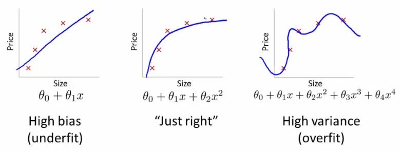
In this section the lecturer examine the relationship between the degree of the polynomial d and the underfitting or overfitting of our hypothesis:

• One need to distinguish whether bias or variance is the problem contributing to bad predictions.
• High bias is underfitting and high variance is overfitting. Ideally, we need to find a golden mean between these two.

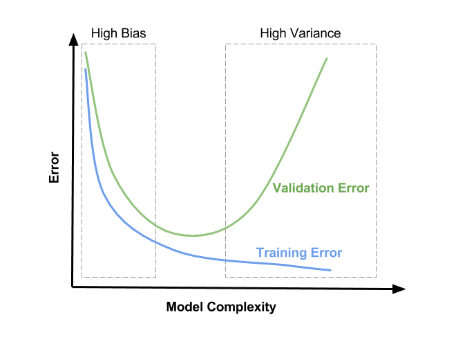
The training error will tend to decrease as we increase the degree d of the polynomial.

At the same time, the cross validation error will tend to decrease as we increase d up to a point, and then it will increase as d is increased, forming a convex curve.

High bias (underfitting): both $J_{train}(\Theta)$ and $J_{CV}(\Theta)$ will be high. Also, $J_{train}(\Theta) \approx J_{CV}(\Theta)$

High variance (overfitting): $J_{train}(\Theta)$ will be low and $J_{CV}(\Theta)$ will be much greater than $J_{train}(\Theta)$

The is summarized in the figure below:

Regularization and Bias/Variance

As λ increases, our fit is like to become more rigid. On the other hand, as λ approaches 0, we tend to over overfit the data. So how do we choose our parameter λ to get it ‘just right’ ? In order to choose the model and the regularization term λ, we need to:

1. Create a list of lambdas (i.e. λ∈{0,0.01,0.02,0.04,0.08,0.16,0.32,0.64,1.28,2.56,5.12,10.24});
2. Create a set of models with different degrees or any other variants.
3. Iterate through the λs and for each λ go through all the models to learn some Θ.
4. Compute the cross validation error using the learned Θ (computed with λ) on the $J_{CV}(Θ)$ without regularization or λ = 0 (as you have regularized already).
5. Select the best combo that produces the lowest error on the cross validation set.
6. Using the best combo Θ and λ, apply it on $J_{test}(Θ)$ to see if it has a good generalization of the problem.

Learning Curves

Experiencing high bias:

Low training set size: causes $J_{train}(Θ)$ to be low and $J_{CV}(Θ)$ to be high.
Large training set size: causes both $J_{train}(Θ)$ and $J_{CV}(Θ)$ to be high with $J_{train}(\Theta) \approx J_{CV}(\Theta)$

If a learning algorithm is suffering from high bias, getting more training data will not (by itself) help much:

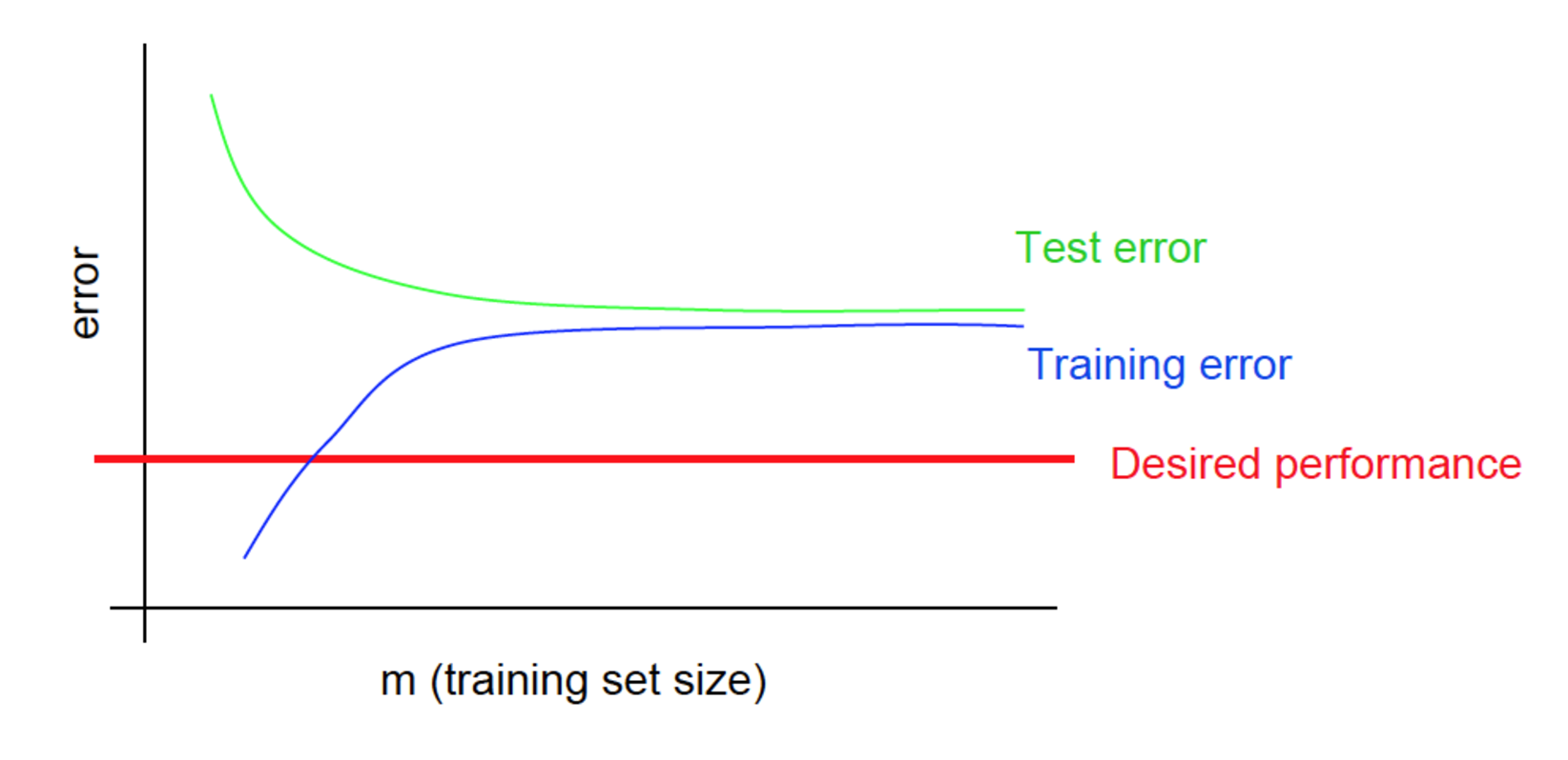
Experiencing high variance:

Low training set size: causes $J_{train}(Θ)$ to be low and $J_{CV}(Θ)$ to be high.
Large training set size: $J_{train}(Θ)$ increases with training set size and $J_{CV}(Θ)$ continues to decrease without leveling off. Also, $J_{train}(\Theta) < J_{CV}(\Theta)$ but the difference between them remains significant:

If a learning algorithm is suffering from high variance, getting more training data is likely to help.

Diagnosing Neural Networks

• A neural network with fewer parameters is prone to underfitting. It is also computationally cheaper.
• A large neural network with more parameters is prone to overfitting. It is also computationally expensive. In this case you can use regularization (increase λ) to address the overfitting.

Using a single hidden layer is a good starting default. You can train your neural network on a number of hidden layers using your cross validation set. You can then select the one that performs best.

Overall

Our decision process can be broken down as follows:

• Getting more training examples: Fixes high variance
• Trying smaller sets of features: Fixes high variance
• Adding features: Fixes high bias
• Adding polynomial features: Fixes high bias
• Decreasing λ: Fixes high bias
• Increasing λ: Fixes high variance.

Model Complexity Effects:

• Lower-order polynomials (low model complexity) have high bias and low variance. In this case, the model fits poorly consistently.
• Higher-order polynomials (high model complexity) fit the training data extremely well and the test data extremely poorly. These have low bias on the training data, but very high variance.
• In reality, we would want to choose a model somewhere in between, that can generalize well but also fits the data reasonably well.

Prioritizing What to Work On

System Design Example:

Given a data set of emails, we could construct a vector for each email in which each entry represents a word. The vector normally contains massive entries gathered by finding the most frequently used words in our data set. A word that exists in the email shall assign its entry to 1 and 0 otherwise. Then we train our algorithm and try to use it to classify if an email is a spam or not.

So how could you spend your time to improve the accuracy of this classifier?

• Collect lots of data (for example “honeypot” project but doesn’t always work)
• Develop sophisticated features (for example: using email header data in spam emails)
• Develop algorithms to process your input in different ways (recognizing misspellings in spam).

It is difficult to tell which of the options will be most helpful.

Error Analysis

The recommended approach to solving machine learning problems is to:

• Start with a simple algorithm, implement it quickly, and test it early on your cross validation data.
• Plot learning curves to decide if more data, more features, etc. are likely to help.
• Manually examine the errors on examples in the cross validation set and try to spot a trend where most of the errors were made.

For example, assume that we have 500 emails and our algorithm misclassifies a 100 of them. We could manually analyze the 100 emails and then try to come up with new cues and features that would help us classify these 100 emails correctly.

It is very important to get error results as a single, numerical value. Otherwise it is difficult/time-consuming to assess your algorithm’s performance.
For example if we try to distinguish between upper and lower case letters and end up getting a 3.2% error rate instead of 3%, then we should avoid using this new feature. Hence, we should try new things, get a numerical performance rate, and based on that decide whether to keep the new feature or not.

Precision and Recall

For skewed data, we are often unable to use tools like error rates to assess a model’s performance. That is because, for instance, if we have a dataset in which 0.5% of them have response 0 and 1 otherwise. Then a complicated model with 1% error rate looks not so good as we can simply predict all of them as 1(which gives a 0.5% error rates). It’s also hard to tell whether a improvement for a model, such as 0.8% to 0.5%, is significant or not.
We therefore need to develop a new tool for this extreme case, that is the Precision and Recall:

	Actually True	Actually False
Predicted True	True positive	False positive
Predicted False	False negative	True negative

$$\text{Precision} = \frac{\text{True positives}}{\text{No. of predicted as positive}} = \frac{\text{True positives}}{\text{True positives + False positives}}$$ $$\text{Recall} = \frac{\text{True positives}}{\text{No. of actual positives}} = \frac{\text{True positives}}{\text{True positives + False negatives}}$$

Trade off between Precision and Recall

High Precision or high Recall? Difficult choice isn’t it! A formula called F score makes it possible to assess the algorithm by a single numerical value:

$$\text{F score} = 2* \ \frac{\text{Precision} * \text{Recall}}{\text{Precision} + \text{Recall}} \in [0, 1]$$

The higher the score, the better the result.