Coursera Machine Learning Week 4-5

Contents: Neural Networks.

Week 4

Neural Networks

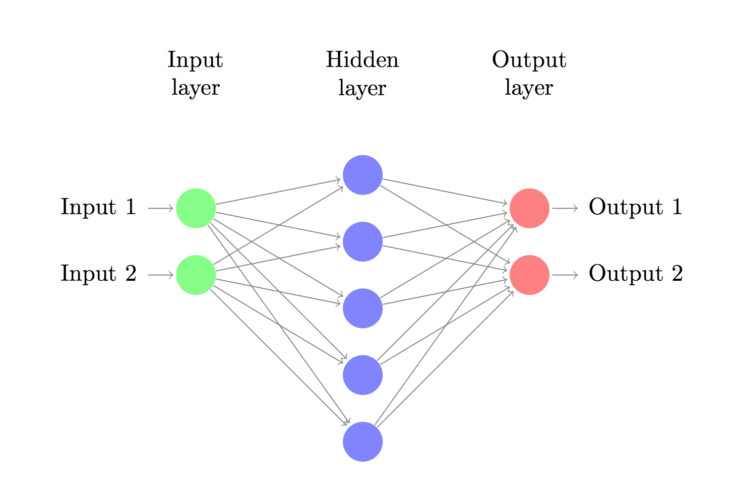
Neurons are computational units that take inputs (dendrites) as electrical inputs (called spikes) that are channeled to outputs (axons). There are also intermediate layers of nodes between the input and output layers called the hidden layers, and the nodes inside are named activation units.

$$\begin{align*}& a_i^{(j)} = \text{"activation" of unit i in layer j} \newline& \Theta^{(j)} = \text{matrix of weights controlling function mapping from layer j to layer j+1}\end{align*}$$

If we had one hidden layer, it would look like:

Let’s say we have a neural metwork with 3 input nodes in layer 1, 3 activation nodes in layer 2, 1 output node in layer 3:

$$\begin{bmatrix}x_0 \newline x_1 \newline x_2 \newline x_3\end{bmatrix}\rightarrow\begin{bmatrix}a_1^{(2)} \newline a_2^{(2)} \newline a_3^{(2)} \newline \end{bmatrix}\rightarrow h_\theta(x)$$

The values for each of the “activation” nodes is obtained as follows:

$$\begin{align*} a_1^{(2)} = g(\Theta_{10}^{(1)}x_0 + \Theta_{11}^{(1)}x_1 + \Theta_{12}^{(1)}x_2 + \Theta_{13}^{(1)}x_3)& \newline a_2^{(2)} = g(\Theta_{20}^{(1)}x_0 + \Theta_{21}^{(1)}x_1 + \Theta_{22}^{(1)}x_2 + \Theta_{23}^{(1)}x_3)& \ \ \ \ \ \ \ \ \ \ \ \ \text{(#)}\newline a_3^{(2)} = g(\Theta_{30}^{(1)}x_0 + \Theta_{31}^{(1)}x_1 + \Theta_{32}^{(1)}x_2 + \Theta_{33}^{(1)}x_3)& \newline \end{align*}$$

This is saying that we compute our activation nodes by using a 3×4 matrix of parameters. We apply each row of the parameters to our inputs to obtain the value for one activation node.

Our hypothesis output is the logistic function applied to the sum of the values of our activation nodes, which have been multiplied by yet another parameter matrix, containing the weights for our second layer of nodes:

$$h_\Theta(x) = a_1^{(3)} = g(\Theta_{10}^{(2)}a_0^{(2)} + \Theta_{11}^{(2)}a_1^{(2)} + \Theta_{12}^{(2)}a_2^{(2)} + \Theta_{13}^{(2)}a_3^{(2)})$$

The dimensions of these matrices of weights is determined as follows:

$$\text{Each layer gets its own matrix of weights, $Θ^{(j)}$.}$$ $$\text{If network has $s_j$ units in layer $j$ and $s_{j+1}$ units in layer $j+1$, then $\Theta^{(j)}$ will be of dimension $s_{j+1} \times (s_j + 1)$.}$$ $$\text{Where the "+1" comes from the "bias nodes", $x_0$ and $Θ^{(j)}_0$ }$$

In other words the output nodes will not include the bias nodes while the inputs will.

Vectorized implementation

For layer j = h and node k, we define a new variable z as:

$$z_k^{(h)} = \Theta_{k,0}^{(h-1)}x_0 + \Theta_{k,1}^{(h-1)}x_1 + \cdots + \Theta_{k,n}^{(h-1)}x_n$$

Therefore the formula in (#) can be rewritten as:

$$\begin{align*}a_1^{(2)} = g(z_1^{(2)}) \newline a_2^{(2)} = g(z_2^{(2)}) \newline a_3^{(2)} = g(z_3^{(2)}) \newline \end{align*}$$

With more newly-defined variables:

$$\begin{align*}x = \begin{bmatrix}x_0 \newline x_1 \newline\cdots \newline x_n\end{bmatrix} \ \ \ \ \ \ &z^{(j)} = \begin{bmatrix}z_1^{(j)} \newline z_2^{(j)} \newline\cdots \newline z_n^{(j)}\end{bmatrix}\end{align*}$$

We then are able to vectorized it further:

$$a^{(j)} = g(z^{(j)}) \ \ ,a^{(j)}\in \mathbb{R}^n$$

Next, we take a’s toward next layer:

$$z^{(j)} = \Theta^{(j-1)} g(z^{(j-1)}) = \Theta^{(j-1)}a^{(j-1)}$$

Here, we multiply our matrix $Θ^{(j−1)}$ with dimensions $s_j ×(n+1)$ (where $s_j$ is the number of our activation nodes) by our vector $a^{j-1}$ with height (n+1). This gives us our vector $z^{(j)}$ with height $s_j$
Overall, the iteration goes like this, and this is also called:

Forward propagation

$$z^{(1)} = \Theta^{(1)}x$$ $$a^{(2)} = g(z^{(1)})$$ $$……$$ $$a^{(j)} = g(z^{(j)})$$ $$z^{(j+1)} = \Theta^{(j)}a^{(j)}$$ $$a^{(j+1)} = g(z^{(j+1)})$$ $$z^{(j+2)} = \Theta^{(j+1)}a^{(j+1)}$$ $$……$$ $$h_\Theta(x) = a^{(??)} = g(z^{(??)})$$

Notice that in the last step and all the assignation of a’s, we are doing exactly the same thing as we did in logistic regression. Adding all these intermediate layers in neural networks allows us to more elegantly produce interesting and more complex non-linear hypotheses.

Example

We can below that the sigmoid function is about 1 when x > 4 (vice versa), this property can help us to develop some example.

Let’s construct a nerual network:

$$\begin{align*}\begin{bmatrix}x_0 \newline x_1 \newline x_2\end{bmatrix} \rightarrow\begin{bmatrix}g(z^{(2)})\end{bmatrix} \rightarrow h_\Theta(x)\end{align*}$$

and fixed the first theta matrix as:

$$\Theta^{(1)} =\begin{bmatrix}-30 & 20 & 20\end{bmatrix}$$

This will cause the output of our hypothesis to only be positive if both inputs are 1. In other words:

$$\begin{align*}& h_\Theta(x) = g(-30 + 20x_1 + 20x_2) \newline \newline & x_1 = 0 \ \ and \ \ x_2 = 0 \ \ then \ \ g(-30) \approx 0 \newline & x_1 = 0 \ \ and \ \ x_2 = 1 \ \ then \ \ g(-10) \approx 0 \newline & x_1 = 1 \ \ and \ \ x_2 = 0 \ \ then \ \ g(-10) \approx 0 \newline & x_1 = 1 \ \ and \ \ x_2 = 1 \ \ then \ \ g(10) \approx 1\end{align*}$$

Therefore we have constructed one of the fundamental operations in computers by using a small neural network rather than using an actual AND gate.

For examples with a hidden layer, please refers to the notes in Examples and Intuitions II

Multiclass Classification

This is done similarly to the one for logistic regression where we use the one-vs-all method. Saying we want to distinguish amongst a car, pedestrian, truck, or motorcycle, then instead of letting hypothesis equals to 1, 2, 3, 4 to correspond to each of them, we set:

$$h_\Theta(x) =\begin{bmatrix}1 \newline 0 \newline 0 \newline 0 \newline\end{bmatrix},\begin{bmatrix}0 \newline 1 \newline 0 \newline 0 \newline\end{bmatrix},\begin{bmatrix}0 \newline 0 \newline 1 \newline 0 \newline\end{bmatrix},\begin{bmatrix}0 \newline 0 \newline 0 \newline 1 \newline\end{bmatrix}$$

So that we can construct a nerual network with 4 output nodes.

Week 5

Cost function

Our cost function for neural networks is going to be a generalization of the one we used for logistic regression:

$$\begin{gather*} J(\Theta) = - \frac{1}{m} \sum_{i=1}^m \sum_{k=1}^K \left[y^{(i)}_k \log ((h_\Theta (x^{(i)}))_k) + (1 - y^{(i)}_k)\log (1 - (h_\Theta(x^{(i)}))_k)\right] + \frac{\lambda}{2m}\sum_{l=1}^{L-1} \sum_{i=1}^{s_l} \sum_{j=1}^{s_{l+1}} ( \Theta_{j,i}^{(l)})^2\end{gather*}$$ $$\begin{align*}\text{where} \ \ \ \ L &= \text{total number of layers in the network} \newline s_l &= \text{number of units (not counting bias unit) in layer} \ l \newline K &= \text{number of output units/classes} \newline h_{\Theta}(x)_k &= \text{a hypothesis that results in the $k^{th}$ output } \end{align*}$$

We have added a few nested summations to account for our multiple output nodes. In the first part of the equation, before the square brackets, we have an additional nested summation that loops through the number of output nodes.

In the regularization part, after the square brackets, we must account for multiple theta matrices. The number of columns in our current theta matrix is equal to the number of nodes in our current layer (including the bias unit). The number of rows in our current theta matrix is equal to the number of nodes in the next layer (excluding the bias unit). As before with logistic regression, we square every term.

Note:

• the double sum simply adds up the logistic regression costs calculated for each cell in the output layer
• the triple sum simply adds up the squares of all the individual Θs in the entire network.
• the i in the triple sum does not refer to training example i

Back propagation

“Backpropagation” is neural-network terminology for minimizing our cost function, just like what we were doing with gradient descent in logistic and linear regression. Our goal is to compute:

$$\min_\Theta J(\Theta)$$

That is, we want to minimize our cost function J using an optimal set of parameters in theta. In this section we’ll look at the equations we use to compute the partial derivative of J(Θ):

$$\dfrac{\partial}{\partial \Theta_{i,j}^{(l)}}J(\Theta)$$

To do so, we use the Back propagation Algorithm:

$$\begin{align*} &\text{Given training set } \lbrace (x^{(1)}, y^{(1)}) \cdots (x^{(m)}, y^{(m)})\rbrace \newline &\text{Set $\Delta_{i,j}^{(l)}: = 0$ for all (l,i,j), (hence you end up having a matrix full of zeros)} \newline\end{align*}$$

---

$$\begin{align*} &\text{For training example t = 1 to m:} \newline &\text{1. Set $a^{(1)} := x^{(t)}$} \newline \newline &\text{2. Perform forward propagation to compute $a^{(l)}$ for l=2,3,…,L} \newline \newline &\text{3. Using $y^{(t)}$, compute $\delta^{(L)} = a^{(L)} - y^{(t)}$} \newline &\text{Where L is our total number of layers and $a^{(L)}$ is the vector of outputs of the activation units for } \newline &\text{the last layer. So our "error values" for the last layer are simply the differences of our actual } \newline &\text{results in the last layer and the correct outputs in y. To get the delta values of the layers before} \newline &\text{the last layer, we can use an equation that steps us back from right to left:} \newline\newline &\text{4. Compute $\delta^{(L-1)}, \delta^{(L-2)},……，\delta^{(2)}$ using $\delta^{(l)} = ((\Theta^{(l)})^T \delta^{(l+1)})\ .* \ g'(z^{(l)})$} \newline &\text{Where $.*$ means element-wise multiplication, and $g'$ is the derivative of the activation } \newline &\text{function g evaluated with the input values given by $z^{(l)}$:} \newline & \ \ \ \ \ \ \ \ \ \ \ \ g'(z^{(l)}) = a^{(l)} .* \ (1 - a^{(l)}) \newline\newline &\text{5. $\Delta_{i,j}^{(l)}:= \Delta_{i,j}^{(l)} + a_j^{(l)}\delta_i^{(l+1)}$, or with vectorization, $\Delta^{(l)} := \Delta^{(l)} + \delta^{(l+1)}(a^{(l)})^T$} \newline \end{align*}$$

---

After finishing the for loop, we update our new Δ matrix:

• $D^{(l)}_{i,j} := \dfrac{1}{m}\left(\Delta^{(l)}_{i,j} + \lambda\Theta^{(l)}_{i,j}\right)$ if j ≠ 0.
• $D^{(l)}_{i,j} := \dfrac{1}{m}\Delta^{(l)}_{i,j}$ if j = 0.

The capital-delta matrix D is used as an “accumulator” to add up our values as we go along and eventually compute our partial derivative. Thus we get:

$$\frac \partial {\partial \Theta_{ij}^{(l)}} J(\Theta)$$

From above we can see Step 4 is doing the most important job, where the $\delta^{(l)}_j$ is actually called the “error” of $a^{(l)}_j$ (unit j in layer l). More formally, the delta values are actually the derivative of the cost function $cost(t) =y^{(t)} \ \log (h_\Theta (x^{(t)})) + (1 - y^{(t)})\ \log (1 - h_\Theta(x^{(t)}))$ (binary classfication case):

$$\delta_j^{(l)} = \dfrac{\partial}{\partial z_j^{(l)}} cost(t)$$

Implementation Note: Unrolling Parameters

In order to use optimizing functions such as “fminunc()” when training the neural network, we will want to “unroll” all the elements and put them into one long vector:

Saying we have $\Theta^{(1)} \in \mathbb{R}^{10×11}, \Theta^{(2)}\in \mathbb{R}^{10×11},\Theta^{(3)}\in \mathbb{R}^{11×1}$

% In order to use optimizing functions such as "fminunc()", 
% we will want to "unroll" all the elements and put them into one long vector:
thetaVector = [ Theta1(:); Theta2(:); Theta3(:); ]

% we can also get back our original matrices from the "unrolled" versions
% as follows:
Theta1 = reshape(thetaVector(1:110),10,11)
Theta2 = reshape(thetaVector(111:220),10,11)
Theta3 = reshape(thetaVector(221:231),1,11)

Gradient Checking

In some case the cost function converges even when the neural network is not learning in the right way. Gradient checking will assure that our backpropagation works as intended. We can approximate the derivative of our cost function with:

$$\dfrac{\partial}{\partial\Theta}J(\Theta) \approx \dfrac{J(\Theta + \epsilon) - J(\Theta - \epsilon)}{2\epsilon}$$

With multiple theta matrices, we can approximate the derivative with respect to $\Theta_j$ as follows:

$$\dfrac{\partial}{\partial\Theta_j}J(\Theta) \approx \dfrac{J(\Theta_1, \dots, \Theta_j + \epsilon, \dots, \Theta_n) - J(\Theta_1, \dots, \Theta_j - \epsilon, \dots, \Theta_n)}{2\epsilon}$$

In matlab we can do it as follows:

epsilon = 1e-4;
for i = 1:n,
  thetaPlus = theta;
  thetaPlus(i) += epsilon;
  thetaMinus = theta;
  thetaMinus(i) -= epsilon;
  gradApprox(i) = (J(thetaPlus) - J(thetaMinus))/(2*epsilon)
end;

A small value for ϵ (epsilon) such as ϵ=0.0001, guarantees that the math works out properly. If the value for ϵ is too small, we can end up with numerical problems.

We previously saw how to calculate the deltaVector. So once we compute our gradApprox vector, we can check that gradApprox ≈ deltaVector. Once you have verified once that your backpropagation algorithm is correct, you don’t need to compute gradApprox again. The code to compute gradApprox can be very slow.

Random Initialization

Initializing all theta weights to zero does not work with neural networks. When we backpropagate, all nodes will update to the same value repeatedly. Instead we can randomly initialize each $\Theta_{ij}^{(l)}$ to a random value between $[-\epsilon,\epsilon]$, then the above formula guarantees that we get the desired bound. In matlab, we can do:

% If the dimensions of Theta1 is 10x11, Theta2 is 10x11 and Theta3 is 1x11.

Theta1 = rand(10,11) * (2 * INIT_EPSILON) - INIT_EPSILON;
Theta2 = rand(10,11) * (2 * INIT_EPSILON) - INIT_EPSILON;
Theta3 = rand(1,11) * (2 * INIT_EPSILON) - INIT_EPSILON;

rand(x,y) is just a function in octave that will initialize a matrix of random real numbers between 0 and 1.

(Note: the epsilon used above is unrelated to the epsilon from Gradient Checking)

Putting it Together

First, pick a network architecture; choose the layout of your neural network, including how many hidden units in each layer and how many layers in total you want to have.

• Number of input units = dimension of features $x^{(i)}$
• Number of output units = number of classes
• Number of hidden units per layer = usually more the better (must balance with cost of computation as it increases with more hidden units)
• Defaults: 1 hidden layer. If you have more than 1 hidden layer, then it is recommended that you have the same number of units in every hidden layer.

Training a Neural Network

1. Randomly initialize the weights
2. Implement forward propagation to get $h_Θ(x^{(i)})$ for any $x^{(i)}$
3. Implement the cost function
4. Implement backpropagation to compute partial derivatives
5. Use gradient checking to confirm that your backpropagation works. Then disable gradient checking.
6. Use gradient descent or a built-in optimization function to minimize the cost function with the weights in theta.

Note that:

• Ideally, you want $h_Θ(x^{(i)}) \approx y^{(i)}$ . This will minimize our cost function. However, keep in mind that J(Θ) is not convex and thus we can end up in a local minimum instead.
• When we perform forward and back propagation, we loop on every training example:

for i = 1:m,
   Perform forward propagation and backpropagation using example (x(i),y(i))
   (Get activations a(l) and delta terms d(l) for l = 2,...,L