Coursera Machine Learning Week 1-3

Contents: Linear Regression, logistic regression, gradient descent and more.

Week 1

Supervised learning problems are categorized into “regression” and “classification” problems. In a regression problem, we are trying to predict results within a continuous output, meaning that we are trying to map input variables to some continuous function. In a classification problem, we are instead trying to predict results in a discrete output. In other words, we are trying to map input variables into discrete categories.

Regression

We can derive this structure by clustering the data based on relationships among the variables in the data.

$$\begin{align*} m &= \text{Number of training examples} \newline x's &= \text{"input" variables / features} \newline y's &= \text{"output" variables / "target" variable} \newline (x^{i}, y^{i}) \ &= i_{th} \ \text{training example} \newline \end{align*}$$

To describe the supervised learning problem slightly more formally, our goal is, given a training set, to learn a function h : X → Y so that h(x) is a “good” predictor for the corresponding value of y. For historical reasons, this function h is called a hypothesis.

cost function (Mean squared error MSE):

$$J(\theta_0, ..., \theta_n) = \dfrac {1}{2m} \displaystyle \sum _{i=1}^m \left (h_\theta (x_{i}) - y_{i} \right)^2$$

Our goal is to minimise the cost function, where one possible approach is gradient descent:

$$\theta_j := \theta_j - \frac{\alpha}{m} \frac{\partial}{\partial \theta_j} J(\theta_0, \theta_1)$$

where j = 0, …, n and α is learning rate.

We keep update θ’s simultaneously until it converge, such that MSE is minimised.
One of the potential issues with this approach is that it may diverge or converge to local minimum(which is not global minimum).

Week 2

Multivariate Linaer Regression

$$\begin{align*}x_j^{(i)} &= \text{value of feature } j \text{ in the }i^{th}\text{ training example} \newline x^{(i)}& = \text{the input (features) of the }i^{th}\text{ training example} \newline m &= \text{the number of training examples} \newline n &= \text{the number of features} \end{align*}$$

hypothesis: $\begin{align*}h_\theta(x) &=\begin{bmatrix}\theta_0 \hspace{1em} \theta_1 \hspace{1em} ... \hspace{1em} \theta_n\end{bmatrix}\begin{bmatrix}x_0 \newline x_1 \newline \vdots \newline x_n\end{bmatrix}= \theta^T x \newline &= \theta_0 + \theta_1x_1 + ... + \theta_nx_n \end{align*}$

Gradient Descent for Multiple Variables:

$$\begin{align*}& \text{repeat until convergence:} \; \lbrace \newline \; & \theta_j := \theta_j - \alpha \frac{1}{m} \sum\limits_{i=1}^{m} (h_\theta(x^{(i)}) - y^{(i)}) \cdot x_j^{(i)} \; & \text{for j := 0...n}\newline \rbrace\end{align*}$$

There are some techiques that could spped up Gradient Descent:

• feature scaling and mean normalization — (working with features)

• Debugging gradient descent: Make a plot with number of iterations on the x-axis. Now plot the cost function, J(θ) over the number of iterations of gradient descent. If J(θ) ever increases, then you probably need to decrease α.

  Automatic convergence test: Declare convergence if J(θ) decreases by less than E in one iteration, where E is some small value such
  as 0.0001. However in practice it’s difficult to choose this threshold value.

  — (working with learning rate)

On other hand, we can combine multiple features into one. For example, we can combine features a and b into a new feature c by taking their product.

Polynomial Regression

Our hypothesis function need not be linear (a straight line) if that does not fit the data well.

We can change the behavior or curve of our hypothesis function by making it a quadratic, cubic or square root function (or any other form).

For instance, we could do $h_\theta(x) = \theta_0 + \theta_1x_1 + \theta_2\sqrt{x_1} + \theta_3x_1^2$

Week 3

Classification

The classification problem is just like the regression problem, except that the values we now want to predict take on only a finite number of discrete values.

Using Linear regression for classification is often not a very good idea, so we need a new learning method for this kind of problem.

This course will focus on binary classification problem, where y only takes 2 values, say 0 or 1.

Logistic Regression

Our new form uses the Sigmoid Function, also called the Logistic Function:

$$\begin{align*} h_\theta (x)& = g ( \theta^T x ) \newline \text{where: } \newline g(z) &= \dfrac{1}{1 + e^{-z}} \newline z &= \theta^T x \end{align*}$$

such that the hypothesis function now satisfies 0 ≤ h ≤ 1, and represents the probability of the output being 1:

$$\begin{align*}& h_\theta(x) = P(y=1 | x ; \theta) = 1 - P(y=0 | x ; \theta) \end{align*}$$

Our hypothesis function will create a decision boundary, which is a line that separates the area where y = 0 and where y = 1

Again, like Polynomial Regression, the input to the sigmoid function can be non-linear.(so the decision boundary may be a open/closed curve instead)

Cost function

We cannot use the same cost function that we use for linear regression because the Logistic Function will cause the output to be wavy, causing many local optima. In other words, it will not be a convex function, where there only exists one global minimum.

Instead, our cost function for logistic regression looks like:

$$\begin{align*}& J(\theta) = \dfrac{1}{m} \sum_{i=1}^m \mathrm{Cost}(h_\theta(x^{(i)}),y^{(i)}) \newline& \text{where the cost for indiviual training example is:} \newline \newline & \mathrm{Cost}(h_\theta(x),y) = -\log(h_\theta(x)) \; & \text{if y = 1} \newline & \mathrm{Cost}(h_\theta(x),y) = -\log(1-h_\theta(x)) \; & \text{if y = 0}\end{align*}$$

And these two functions looks like:

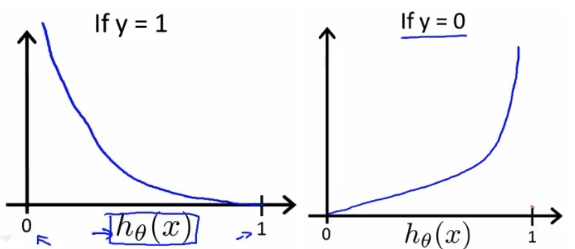
so that these have the following properties:

$$\begin{align*}& \mathrm{Cost}(h_\theta(x),y) = 0 \text{ if } h_\theta(x) = y \newline & \mathrm{Cost}(h_\theta(x),y) \rightarrow \infty \text{ if } y = 0 \; \mathrm{and} \; h_\theta(x) \rightarrow 1 \newline & \mathrm{Cost}(h_\theta(x),y) \rightarrow \infty \text{ if } y = 1 \; \mathrm{and} \; h_\theta(x) \rightarrow 0 \newline \end{align*}$$

And actually, we can compress our cost function’s two conditional cases into one case:

$$\mathrm{Cost}(h_\theta(x),y) = - y \; \log(h_\theta(x)) - (1 - y) \log(1 - h_\theta(x))$$

Therefore our entire cost function is as follows:

$$\begin{align*} J(\theta) = - \dfrac{1}{m} \sum_{i=1}^m [y^{(i)}\log(h_\theta(x^{(i)})) + (1 - y^{(i)})\log(1 - h_\theta(x^{(i)}))] \end{align*}$$

Or, in vectorized implementation:

$$\begin{align*} & J(\theta) = \frac{1}{m} \cdot \left(-y^{T}\log(h)-(1-y)^{T}\log(1-h)\right) \newline &\text{where} \; \; h = g(X\theta)\end{align*}$$

Gradient Descent

The Gradient Descent procedure for logistic regression looks suprisingly similar with linear regression:

$$\begin{align*} & Repeat \; \lbrace \; \theta_j := \theta_j - \frac{\alpha}{m} \sum_{i=1}^m (h_\theta(x^{(i)}) - y^{(i)}) x_j^{(i)} \rbrace \end{align*}$$

Or, in vectorized implementation:

$$\begin{align*} \; \theta := \theta - \frac{\alpha}{m} X^{T}(g(X\theta) - y) \end{align*}$$

Advanced optimization techniques

There are more sophisticated, faster ways to optimize θ that can be used instead of gradient descent, eg:

• Conjugate gradient
• BFGS
• L-BFGS

To use these

function [jVal, gradient] = costFunction(theta)
  jVal = [...code to compute J(theta)...];
  gradient = [...code to compute derivative of J(theta)...];
end;

Then we can use octave’s fminunc() optimization algorithm along with the optimset() function that creates an object containing the options we want to send to fminunc():

options = optimset('GradObj', 'on', 'MaxIter', 100);
initialTheta = zeros(2,1);
   [optTheta, functionVal, exitFlag] = fminunc(@costFunction, initialTheta, options);

Multiclass Classification

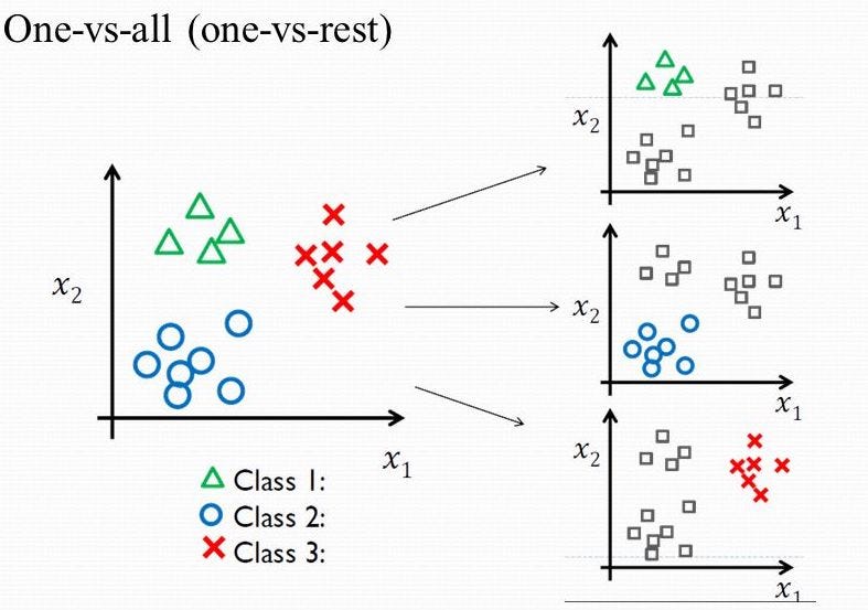
For now we have y = {0,1…n}, one way we can choose is to divide our problem into n+1 binary classification problems; in each one, we choose one class and then lumping all the others into a single second class and then applying binary logistic regression, and then use the hypothesis that returned the highest value (probability)as our prediction, namely pick the class that maximizes the hypothesises, mathematically:

$$\begin{align*}& y \in \lbrace0, 1 ... n\rbrace \newline& h_\theta^{(0)}(x) = P(y = 0 | x ; \theta) \newline& h_\theta^{(1)}(x) = P(y = 1 | x ; \theta) \newline& \cdots \newline& h_\theta^{(n)}(x) = P(y = n | x ; \theta) \newline& \mathrm{prediction} = \max_i( h_\theta ^{(i)}(x) )\newline\end{align*}$$

The following image shows an example of 3 classes:

Overfitting

Overfitting is caused by a hypothesis function that fits the available data but does not generalize well to predict new data. This terminology is applied to both linear and logistic regression. There are two main options to address the issue of overfitting:

(1) Reduce the number of features

• Manually select which features to keep.
• Use a model selection algorithm (studied later in the course).

(2)Regularization

• Keep all the features, but reduce the magnitude of parameters
• Regularization works well when we have a lot of slightly useful features.

The way that to reduce the influence of parameters is to modify our cost function by introducing an additonal term:

$$\min_\theta \frac{1}{2m} \sum_{i = 1}^{m} ((h_{\theta}(x^{(i)}) - y^{(i)})^2 + \lambda \sum_{i = 1}^n \theta_j^2)$$

where λ is the regularization parameter. It determines how much the costs of our theta parameters are inflated.

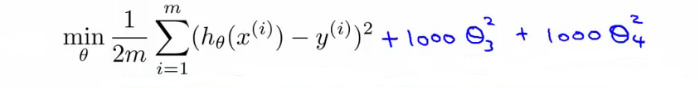
Or, if we want to eliminate a few parameters instead of all of them, just simply inflate the cost of those parameters. For example:

Suppose we penelize and make $\theta_3,\theta_4$ really small

We can apply regularization to both linear regression and logistic regression. We will approach linear regression first:

Regularized Linear Regression

For gradient descent, we will modify our gradient descent function:

$$\begin{align*} & \text{Repeat}\ \lbrace \newline & \ \ \ \ \theta_0 := \theta_0 - \alpha\ \frac{1}{m}\ \sum_{i=1}^m (h_\theta(x^{(i)}) - y^{(i)})x_0^{(i)} \ \ (\text{no need to penalize }\theta_0) \newline & \ \ \ \ \theta_j := \theta_j - \alpha\ \left[ \left( \frac{1}{m}\ \sum_{i=1}^m (h_\theta(x^{(i)}) - y^{(i)})x_j^{(i)} \right) + \frac{\lambda}{m}\theta_j \right] &\ \ \ \ \ \ \ \ \ \ j \in \lbrace 1,2...n\rbrace\newline & \rbrace \end{align*}$$

The new added term performs our regularization. We can also write the function as:

$$\theta_j := \theta_j(1 - \alpha\frac{\lambda}{m}) - \alpha \frac{1}{m}\ \sum_{i=1}^m (h_\theta(x^{(i)}) - y^{(i)})x_j^{(i)}$$

The first term in the above equation, 1 - αλ/m will always be less than 1. Intuitively you can see it as reducing the value of by some amount on every update. Notice that the second term is now exactly the same as it was before.

For Normal Equation, please refer to the reading page for details.

Regularized Logistic Regression

Regularization for logistic regression is similar to the previous one, where we introduce the exactly same term to the cost function as before:

$$J(\theta) = - \frac{1}{m} \sum_{i = 1}^m \left[ y^{(i)}\log(h_\theta(x^{(i)})) + (1 - y^{(i)})\log(1 - h_\theta(x^{(i)}))\right] + \frac{\lambda}{2m} \sum_{i = 1}^n \theta_j^2 \ \ \ (\theta_0\text{ is skipped})$$

and then the gradient descent function (procedure) looks exactly the same as the one for linear regression.